I can’t say that I had the honor of making that acronym - that goes to Prof. Slocum - but I did have the honor of actually designing them.
FPGAs are bi-weekly assignments in 2.70 that involve building a contraption of our choice. The only restraint is that we we demonstrate some fundamental principle of engineering - and, of course, that we do the math.
FPGA 1: Finicky Preload with Great Applications
Have you ever counter-rotated two nuts to make a locknut? That question was rhetorical - everyone does that. But is it actually effective?
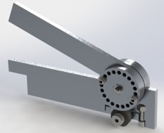
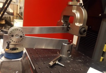
Our first FPGA was an attempt to quantify the actual strength of these preloaded “locknuts”. We first created an analytical model of two nuts held together.
(click to see code)
%% FPGA 1

%% parameters
E = 200 * 10^9; %steel 200 GPa
l = 1/20 * 0.0254; %lead = 1/20 in
L = 7/32*2 * 0.0254; %length of assemble (m)
u = 0.5; % coefficient of friction
r = 1/8 * 0.0254; %radius of bolt

%% derived parameters
A = (((7/16)/2)^2 *pi - ((1/4)/2)^2 *pi) * 0.0254^2; % m^2 front area of nut

%% Do calculation
f1 = @computeForce;
f2 = @computeTorque;

%% Function
% Put in equations form
function force = computeForce(original, final)
    A = (((7/16)/2)^2 *pi - ((1/4)/2)^2 *pi) * 0.0254^2; % m^2 front area of nut
    strain = ((final - original)/original)/2;
    E = 190 * 10^9;
    stress = strain*E;
    force = stress * A;
end
function torque = computeTorque(preload)
    u = 0.5;
    r = 1/8 * 0.0254;
    torque = preload*sind(75)*u*r;
end
We then put our tester-gadget into an Instron to see how our predictions lined up with reality. When using spring washers, our predictions were suprisingly accurate (within 22% in the worst trial) - but when directly mashing the nuts together, our model broke down. Our quest to fix this led to us realizing that bolt tensioning is a science within itself!
FPGA 2: Figure Pondering Grading of Assignment
Our second FPGA was an attempt to make a bistable switch - but not just any switch. We wanted it to be the most satisfying switch in existence.
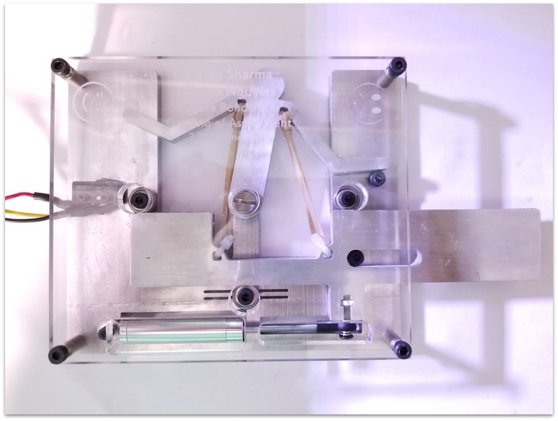
Our bistable switch features a special 2D arrangement of springs that allows it to snap between two positions with hysterises in a predictable fashion. The static behavior of the system was calculated using a potential energy well based solver.
(click to see code)
import numpy as np
from mpl_toolkits.mplot3d import Axes3D
import matplotlib.pyplot as plt
from matplotlib import cm
from matplotlib.ticker import LinearLocator, FormatStrFormatter


# input parameters (all in mm | radians | N/mm)

p2s = 22  # pivot to slider distance
pl = 44  # pivot length
prom = np.pi / 6  # pivot range of motion (total)
lrom = 25  # slider range of motion (total)
ss = 44  # spring seperation
k = 1.3 / 30  # spring constant
srl = 30  # spring resting length
so = 15  # spring pivot seperation
precision = 100  # number of points to evaluate

# equation derived from matlab


def energy(pa, delta):
    """
    equation source:
    pc = [-pl*np.np.cos(pa), pl*np.np.sin(pa)] % pivot attachment point coords

    tpc = [p2s, ss/2 + delta] % top spring attachment coords

    bpc = [p2s, -ss/2 + delta] % bottom spring attachment coords

    tsl = norm(pc - tpc) % top spring length

    bsl = norm(pc - bpc) % bottom spring length

    tse = (tsl - srl)*k % top spring energy

    bse = (bsl - srl)*k % bottom spring energy

    te = tse + bse % total energy

    matlabs symbolic stuff is way easier lol

    delta -> shift in spring origin
    pa -> angle of pivot

    """
    return (k*(srl - (abs(delta - ss/2 + so*np.cos(pa) - pl*np.sin(pa))**2 + abs(p2s + pl*np.cos(pa) + so*np.sin(pa))**2)**(1/2))**2)/2 + (k*(srl - (abs(delta + ss/2 - so*np.cos(pa) - pl*np.sin(pa))**2 + abs(p2s + pl*np.cos(pa) - so*np.sin(pa))**2)**(1/2))**2)/2


# create map of energy


energy_map_func = np.vectorize(energy)

deltas = np.linspace(-lrom / 2, lrom / 2, precision)

pas = np.linspace(-prom / 2, prom / 2, precision)

pas_Y, deltas_X = np.meshgrid(pas, deltas)

energies = energy_map_func(pas_Y, deltas_X)

# map forward stroke
# starting energy


def generate_path(flipped):
    angles_indexes = [energies[0].argmin()]
    if flipped:
        angles_indexes = [energies[energies.shape[0] - 1].argmin()]
    steps = range(1, energies.shape[0])
    if flipped:
        steps = reversed(steps)
    for i in steps:
        c_angle = angles_indexes[-1]
        while (c_angle > 0):
            if energies[i][c_angle] > energies[i][c_angle - 1]:
                c_angle = c_angle - 1
            else:
                break

        while (c_angle < len(energies[i]) - 1):
            if energies[i][c_angle] > energies[i][c_angle + 1]:
                c_angle = c_angle + 1
            else:
                break

        angles_indexes.append(c_angle)

    path_deltas = deltas
    if flipped:
        path_deltas = [i for i in reversed(deltas)]
    path_pas = [pas[i] for i in angles_indexes]

    path_energies = [energies[i][j]
                     for i, j in zip(range(precision), angles_indexes)]
    if flipped:
        path_energies = [energies[i][j] for i, j in zip(
            reversed(range(precision)), angles_indexes)]

    return (path_deltas, path_pas, path_energies)


fig = plt.figure()
ax = fig.gca(projection='3d')

# Plot the surface.
surf = ax.plot_surface(deltas_X, pas_Y, energies, alpha=0.5,
                       cmap=cm.coolwarm, linewidth=0, antialiased=False)

line_forward = ax.plot(*generate_path(False), linewidth=3, label="Forward Crank Path")
line_backward = ax.plot(*generate_path(True), linewidth=3, label="Backwards Crank Path")

# Customize the z axis.
ax.zaxis.set_major_locator(LinearLocator(6))
ax.zaxis.set_major_formatter(FormatStrFormatter('%.01f'))
ax.set_xlabel("Slider Position")
ax.set_ylabel("Crank Angle")
ax.set_zlabel("Elastic Energy Stored")
ax.legend()
# Add a color bar which maps values to colors.
fig.colorbar(surf, shrink=0.5, aspect=5)

plt.show()
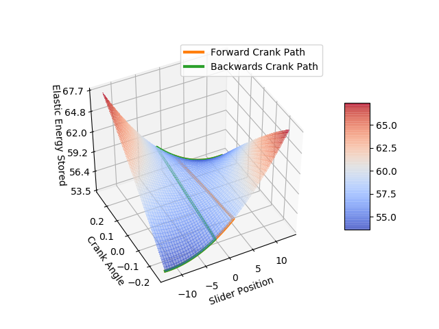
This gave us a nice idea of how the switch would move over its range of motion. The final test showed that our model had only 16% error - most of which came from errors in measuring the resting length of our springs.
FPGA 3: Flexures Put in Ghastly Applications
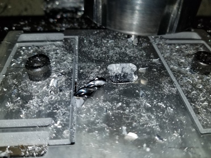
Flexures are wonderful, but they’re not always easy to make. Their very nature means that they tend to move around as you machine them. Most people solve this by simply…not machining them. But what if you did?
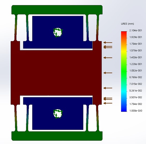
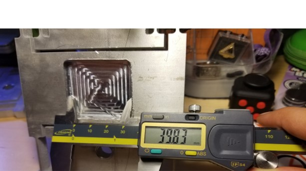
For this FPGA, we tried to quantify how bad tolerances would be if you tried to machine a pocket in a folded-stage flexure. A lot of tuning was needed to get the damn thing to cut in the first place. A lot of punishment was taken every time we messed up :c
Our final model predicted our tolerances to be off by 0.08mm - and our final measurements confirmed this to be accurate (although our measurement techniques could surely be improved).
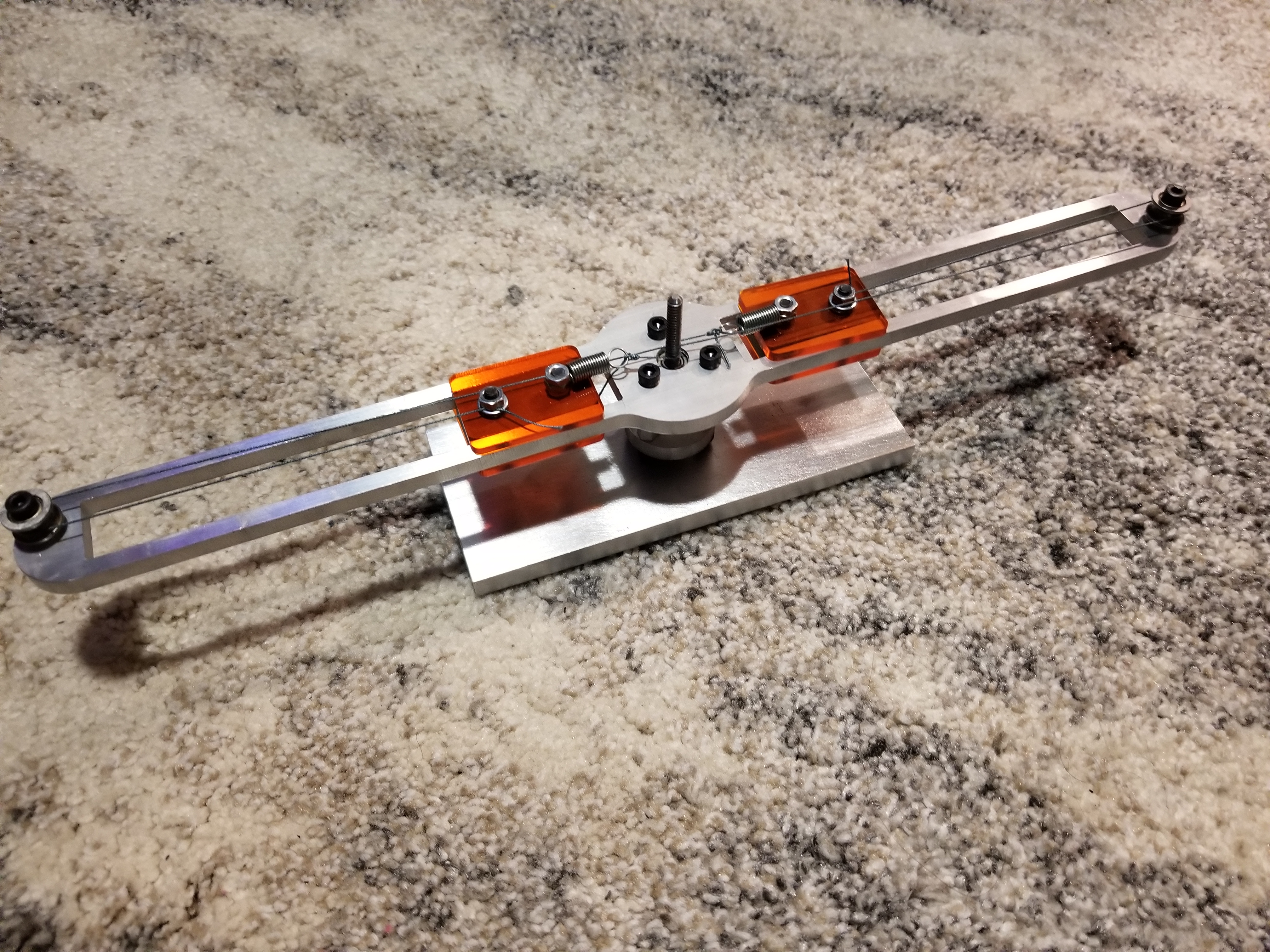
FPGA 4: Freaky Pulleys Going Axially
Overhead cranes typically use large steel I-beams upon which steel rollers glide. Why not make it more like a zipline? Well, that would just result in the rope sagging. Why not use rope sagging to your advantage?
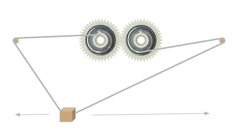
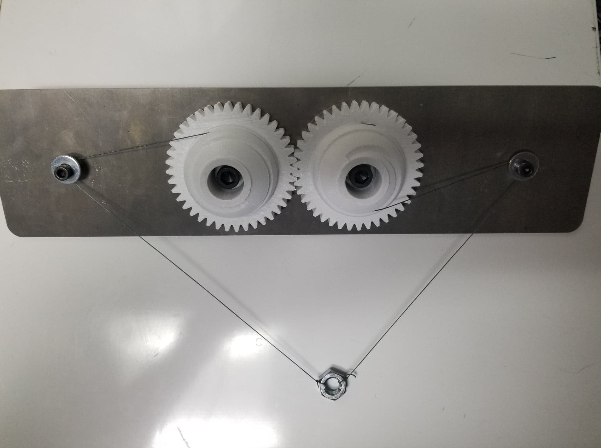
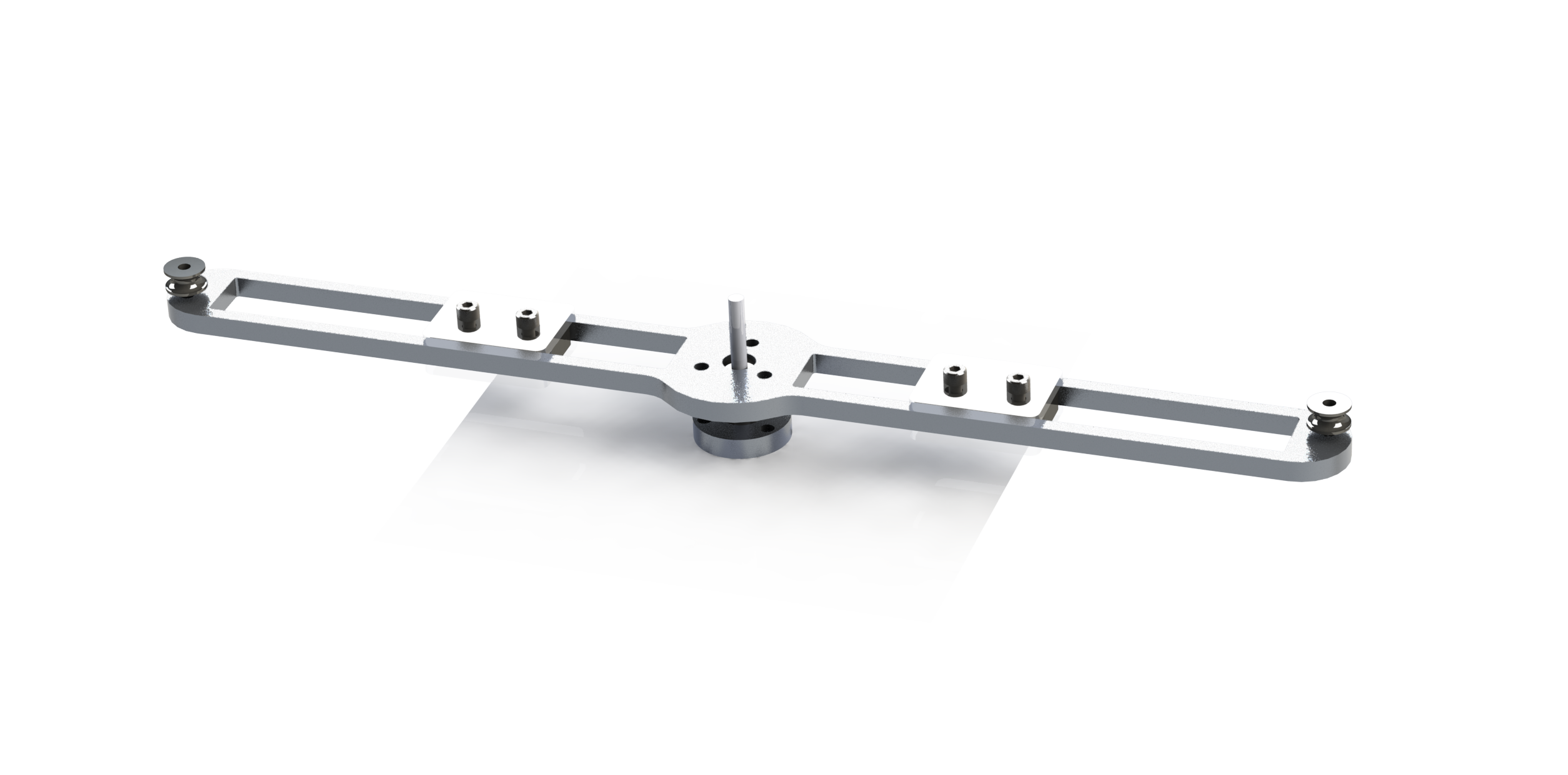
The basic concept was to have two nonlinear winches synchronized together by gears. When one winch releases rope, the other winch takes up rope at the exact rate needed to keep a hanging object moving along a straight line. Tricky, but possible.
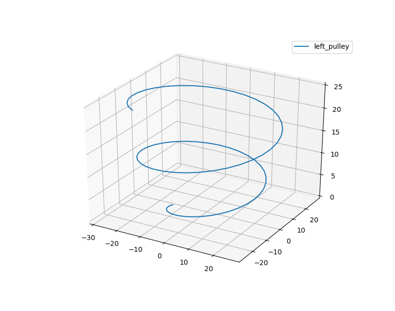
A giant pile of python code and math was used to generate a parametric path through space that represented the shape of the winch.
(click to see code)
import numpy as np
import matplotlib.pyplot as plt
from mpl_toolkits.mplot3d import Axes3D

# input parameters
a = 15  # ratio of pulley angle (radians) to x distance traveled (mm)
H = 100  # distance between pulley and object (mm)
W = 300  # distance between pulleys (mm)
x_padding = 50  # padding between x travel and pulley spacing (mm)
pulley_height = 25  # width of pulley (mm)

# resolution
num_points = 75
# derived figures
x_min = x_padding
x_max = W - x_padding

xs = np.linspace(x_min, x_max, num_points)
thetas = xs / a
pitch = pulley_height / (thetas[-1] - thetas[0])

ds = np.sqrt(np.square(2 * xs * a) / (np.square(xs) + np.square(H)) - np.square(pitch))

# exporting to solidworks curve format

p_x_left = np.cos(thetas) * ds
p_x_right = -np.cos(thetas) * ds
p_y_left = np.sin(thetas) * ds
p_y_right = np.sin(thetas) * ds
p_z_left = np.linspace(0, pulley_height, num_points)
p_z_right = np.linspace(pulley_height, 0, num_points)


# previewing helix shape
fig = plt.figure()
ax = fig.gca(projection='3d')
ax.plot(p_x_left, p_y_left, p_z_left, label='left_pulley')
# ax.plot(p_x_right, p_y_right, p_z_right, label='right_pulley')
ax.legend()

plt.show()


# saving path to file
with open('output_left.sldcrv', 'w') as file:
    output = '\n'.join(' '.join((str(x), str(y), str(z)))
                       for x, y, z in np.vstack((p_x_left, p_y_left, p_z_left)).T)
    file.write(output)

with open('output_right.sldcrv', 'w') as file:
    output = '\n'.join(' '.join((str(x), str(y), str(z)))
                       for x, y, z in np.vstack((p_x_right, p_y_right, p_z_right)).T)
    file.write(output)
The final pulley system - despite all of our expectations - somehow worked as expected! Only a few nonlinearities were observed (mostly due to improper assembly).
FPGA 5: Figure Pulling Great mAss
When hit, a tetherball initially starts wrapping around the poll slowly but speeds up as it winds inwards. This is due to a decreasing moment of inertia and conserved energy. What would a flywheel built to mimick this look like?
A small arm with two counterbalanced weights spins on a pivot. The spinning of the arm causes the two weights to be simultaneously winched together. Predicting how the speed would change as a result was suprisingly difficult and required my partner to write a custom Euler-Lagrange simulator.
(click to see code)
function simulate_leg()

    %% Definte fixed paramters (obtained from CAD)
    m1 =.02 + .210;         m2 =.0225;
    m3 = .004;              m4 = .017;
    I1 = 45.389 * 10^-6;    I2 = 22.918 * 10^-6;
    I3 = 3.2570 * 10^-6;    I4 = 22.176 * 10^-6;
    l_OA=.011;              l_OB=.042;
    l_AC=.096;              l_DE=.096;
    l_O_m1=0.0364;          l_B_m2=0.040;
    l_A_m3=1/2 * l_AC;      l_C_m4=1/2 * (l_DE+ l_OB-l_OA);
    g = 9.81;

    %% Parameter vector
    p   = [m1 m2 m3 m4 I1 I2 I3 I4 l_O_m1 l_B_m2 l_A_m3 l_C_m4 l_OA l_OB l_AC l_DE g]';

    %% Perform Dynamic simulation
    tspan = [0 2];
    z0 = [-pi/4; pi/2; 0; 0];
    opts = odeset('AbsTol',1e-8,'RelTol',1e-6);
    sol = ode45(@dynamics,tspan,z0,opts,p);

    %% Compute Energy
    E = energy_leg(sol.y,p);
    figure(1); clf
    plot(sol.x,E);xlabel('Time (s)'); ylabel('Energy (J)');

    %% Compute foot position over time
    rE = zeros(2,length(sol.x));
    for i = 1:length(sol.x)
        rE(:,i) = position_foot(sol.y(:,i),p);
    end

    w =100;
    % Plot desired and actuatl foot trajectories
    figure(2); clf;
    plot(sol.x,rE(1,:),'r','LineWidth',2)
    hold on
    plot(sol.x,0.025 * cos(w*sol.x) ,'r--');
    plot(sol.x,rE(2,:),'b','LineWidth',2)
    plot(sol.x,-.125+0.025*sin(w*sol.x) ,'b--');

    xlabel('Time (s)'); ylabel('Position (m)'); legend({'x','x_d','y','y_d'});

    %% Animate Solution
    figure(3); clf;
    hold on

    %% Optional, plot foot target information
    % Target traj. Q 1.6
    plot( .025*cos(0:.01:2*pi), -.125+.025*sin(0:.01:2*pi),'k--');

    animateSol(sol,p);
end

function tau = control_law(t,z,p)
    % Controller gains, Update as necessary for Problem 1
    K_x = 40; % Spring stiffness X
    K_y = 40; % Spring stiffness Y
    D_x = 4;  % Damping X
    D_y = 4;  % Damping Y

    % Desired position of foot is a circle
    w   = 30;
    rEd = [0 -.125 0]' + .025*[cos(w*t) sin(w*t) 0]'; % Desired position of foot
    vEd = .025*[-sin(w*t)*w cos(w*t)*w 0]'; % Desired velocity of foot

    rE = position_foot(z,p);
    vE = velocity_foot(z,p);
    J  = jacobian_foot(z,p);

    % Compute virtual foce
    f  = [K_x * (rEd(1) - rE(1) ) - D_x * (vE(1) - vEd(1) ) ;
          K_y * (rEd(2) - rE(2) ) - D_y * (vE(2) - vEd(2) ) ];

    % Map to joint torques
    tau = J' * f;
end

function tau = control_law_extended(t,z,p)
 % Controller gains, Update as necessary for Problem 1
    K_x = 40; % Spring stiffness X
    K_y = 40; % Spring stiffness Y
    D_x = 4;  % Damping X
    D_y = 4;  % Damping Y

    % Desired position of foot is a circle
    w   = 100;
    rEd = [0 -.125 0]' + .025*[cos(w*t) sin(w*t) 0]'; % Desired position of foot
    vEd = .025*[-sin(w*t)*w cos(w*t)*w 0]'; % Desired velocity of foot
    aEd = [-.025*w^2*cos(t*w) -.025*w^2*sin(w*t)]';

    rE = position_foot(z,p);
    vE = velocity_foot(z,p);
    J  = jacobian_foot(z,p);
    dJ = jacobian_dot_foot(z,p);

    %Compute dynamic coefficients
    M = A_leg(z,p);
    lambda = inv(J')*M*inv(J);
    V = Corr_leg(z,p);
    mu = inv(J')*V-lambda*dJ*z(3:4);
    G = Grav_leg(z,p);
    rho = inv(J')*G;


    % Compute virtual foce
    f  = [K_x * (rEd(1) - rE(1) ) - D_x * (vE(1) - vEd(1) ) ;
          K_y * (rEd(2) - rE(2) ) - D_y * (vE(2) - vEd(2) ) ];

    f_new = f + lambda*aEd + rho;
    % Map to joint torques
    tau = J' * f_new;
end


function dz = dynamics(t,z,p)
    % Get mass matrix
    A = A_leg(z,p);

    % Compute Controls
    tau = control_law_extended(t,z,p);

    % Get b = Q - V(q,qd) - G(q)
    b = b_leg(z,tau,p);

    % Solve for qdd.
    qdd = A\b;
    dz = 0*z;

    % Form dz
    dz(1:2) = z(3:4);
    dz(3:4) = qdd;
end

function animateSol(sol,p)
    % Prepare plot handles
    hold on
    h_OB = plot([0],[0],'LineWidth',2);
    h_AC = plot([0],[0],'LineWidth',2);
    h_BD = plot([0],[0],'LineWidth',2);
    h_CE = plot([0],[0],'LineWidth',2);


    xlabel('x'); ylabel('y');
    h_title = title('t=0.0s');

    axis equal
    axis([-.2 .2 -.3 .1]);

    %Step through and update animation
    for t = 0:.01:sol.x(end)
        % interpolate to get state at current time.
        z = interp1(sol.x',sol.y',t)';
        keypoints = keypoints_leg(z,p);

        rA = keypoints(:,1); % Vector to base of cart
        rB = keypoints(:,2);
        rC = keypoints(:,3); % Vector to tip of pendulum
        rD = keypoints(:,4);
        rE = keypoints(:,5);

        set(h_title,'String',  sprintf('t=%.2f',t) ); % update title

        set(h_OB,'XData',[0 rB(1)]);
        set(h_OB,'YData',[0 rB(2)]);

        set(h_AC,'XData',[rA(1) rC(1)]);
        set(h_AC,'YData',[rA(2) rC(2)]);

        set(h_BD,'XData',[rB(1) rD(1)]);
        set(h_BD,'YData',[rB(2) rD(2)]);

        set(h_CE,'XData',[rC(1) rE(1)]);
        set(h_CE,'YData',[rC(2) rE(2)]);

        pause(.01)
    end
end
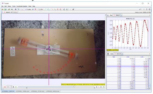
Once it was built, we used Tracker to see whether our observations matched up with our predictions. Parasitic frictional losses ended up thwarting our model… but we could still clearly see the device speeding up over time!
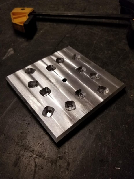
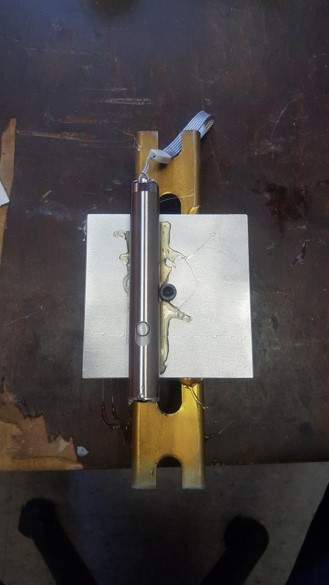
FPGA 6: Fixturing for Precise Gadget Alignment
Kinematic couplings are great for creating repeatable fixtures, but things get weird when you try to have multiple orientations. Undercontrained/overcontrained/undesired orientations crop up when you try to place multiple KCs around one axis. How do you get around this?
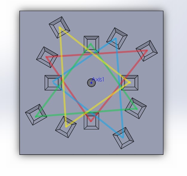
If the coupler locations are offset properly, you can get a coupler that locks in place at an arbitrary number of locations (with no invalid configurations!)
We predicted that there would be some amount of angular error in our coupler (specifically, a max deviation of 1.61e-7 m). We tried testing this using a laser pointer mounted to the top and aimed down a 127ft hallway…
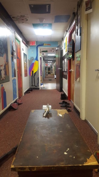
…and we couldn’t measure anything! We believe that the brinelling of the KC grooves might have made this more repeatable than we originally thought!